Wednesday, September 18, 2013
4:13 a.m. (one of those nights…)
Hey everybody! It’s super early Wednesday morning and I woke up and am having trouble falling back asleep. There are two things that make me fall asleep… writing weather blogs and reading the Bible. I’m not religious, I just want to read it because I’m curious about what it has to say and how this has been interpreted by people around the world, especially those in politics. I don’t mean to offend anybody, but it’s really boring… I haven’t gotten out of Genesis yet. That doesn’t make the Bible any less fascinating… it just means that it’s not exactly the most riveting text in the world.
I heard about the Colorado floods when I was moving into my new house. I didn’t have much time to write about them or even study them in detail, but in this post, I’ll give an overview of what happened and why it happened. So without further ado, let’s get to it!
I still remember Seattle’s rainiest day ever recorded. It was October 20, 2003, and I was a fifth-grader at McGilvra Elementary in Madison Park. We had a “rainy-day recess,” and all of our activities were to take place either inside the school gymnasium or under a covered area with basketball hoops and such right outside of it. There were two “portables” (classrooms outside the main school that were built so the school could accommodate more students) that had recently been built outside the school by the gym, and these were on the cusp of being flooded due to a storm drain that had stopped functioning near them. The day afterwards, my mom, my brother and I went on an expedition to find some remaining puddles and came across a small lake in an area near the arboretum that had poor drainage. A couple days later, I went fishing with my dad in Puget Sound and saw logs deposited by the outflow of the region’s rivers scattered outside the Edmonds marina.
I also remember one of the heaviest downbursts of rain ever recorded in Seattle. It was around 4:40 p.m. on Thursday, December 14, 2006 when I began to hear a long, consistent roar outside. I went out to check and witnessed the heaviest rainfall rates I had ever seen in my life. The ground was saturated from the previous November, which was the wettest month on record for many places (including Seattle), and several inches that had fallen since Monday. The ground could not absorb any more water, so the rain from this brief squall turned roads into rivers and even tragically drowned a woman living in Madison Valley, a bowl-shaped region that was among the hardest hit by the storm. My very primitive Lacrosse rain gauge measured rainfall rates of 1.88 inches per hour, and they likely reached over 2 inches per hour for brief periods of time. Those two events stick out very clearly in my mind, and by combining the massive amount of rainfall on the 20th with the massive rates on the 14th, I am able to gain an inkling of perspective on the biblical amounts of rain received in Boulder on the 20th.
Between the afternoon of Monday, September 9 and Friday, September 13, much of the Front Range of Colorado saw unprecedented amounts of rain and associated flash flooding. Boulder was one of the areas hardest hit, receiving 14.62 inches during this time period with 9.08 inches on Thursday, September 12 alone. To make matters even flash-floodier, most of this rain occurred in a couple hours. The previous record for total daily rainfall in Boulder, an impressive 4.80 inches on July 31, 2013, was nearly doubled.
And on that note, I’m hitting the hay. It is 5:59 a.m., and I’ve done a little storytelling and a lot of research that will hopefully make the rest of this post go a little quicker. I’m not Bible-sleepy, but I’m a fair bit more relaxed. 😉
_________________________________________________
Alright. It is 10 hours and 22 minutes later, and I’m ready to write again. I just got back from a strenuous workout, but I’m not quite tired enough to begin my ritualistic afternoon nap. Thankfully, I got the two B’s… Blogger and Bible, and I’ll choose the former.
One note on the pictures below… most of this content was taken from other people’s blogs on the Colorado floods. The pictures below are in the public domain, but I still give credit to the people from which I got the pictures from. I’m adept at obtaining pictures of any sort to describe Pacific Northwest weather because I do it all the time, but I’m simply not familiar with places to get the types of charts and imagery that are shown below.
Now that that’s out of the way, let’s take a look at how it all started.
We had a setup here that was actually pretty darn similar to a setup that brought intense rains to Alberta earlier this summer. The 500 millibar height chart below shows the configuration of the atmosphere on June 20, 2013 at the height of the event. High pressure in northern Alberta prevented a low-pressure system from passing eastward across the country, and since air flows into areas of low pressure, warm, humid air with origins east of the Rockies flowed westward and produced incredible amounts of orographic precipitation as it encountered the topography of the Rockies.
 |
| NWS Upper level analysis of the weather pattern leading to Alberta flooding as of 5 a.m. PDT, Thu 20 Jun 2013. Retrieved from TheWeatherNetwork.com. Chart URL: http://www.theweathernetwork.com/news/articles/colorado-flooding-echoes-of-alberta-/12914/ |
Now, fast-forward three months and you have a very similar scenario setting up further south along the eastern edge of the Rockies.
 |
| NWS Upper level analysis of the weather pattern leading to Colorado flooding as of 5 a.m. PDT, Thu 12 Sep 2013. Retrieved from TheWeatherNetwork.com. Chart URL: http://www.theweathernetwork.com/news/articles/colorado-flooding-echoes-of-alberta-/12914/ |
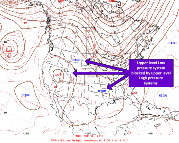
Again, you’ve got a moist, slow-moving low pressure system to the west that has its eastward progress slowed by a large area of high pressure over Canada. It’s essentially the same pattern shifted to the south. Again, this low was responsible for steering air east of the Rockies, in this case directly from the Gulf of Mexico, northwestward into Colorado. This event occurred around the annual peak of sea-surface-temperatures in the Gulf of Mexico, and the air directed into the area had incredible amounts of moisture and heat energy within it. When that air collided into the Front Range, well, you know the rest.
The chart below shows balloon soundings from the Denver area around the time of the big floods. It shows a lot of things, and all are very useful in their own special ways. I want to you take a particularly close look at two things, though. The first is the total Precipitable Water (PW) value, which is located on the bottom left of the chart under “Parcel.” These values are a measure of how much moisture in the atmosphere. More specifically, they measure how much water would precipitate (fall towards the ground) if all the water vapor in a column of the atmosphere was condensed. Since this value is 1.15 inches, the water vapor alone within the column of air sampled by the balloon would amount to 1.15 inches of rain. That’s a LOT of moisture. Additionally, the level of moisture was extremely deep. The red and green lines represent the temperature and dew point, respectively, throughout the atmosphere. They are essentially the same all the way up to the 500mb level, which is approximately 18,000 feet in the atmosphere. That’s INSANE.The top three highest PW values ever recorded in September at Denver since records began in 1948 occurred over the 12-13th, and they completely overshadowed anything that had ever been seen before.
1.33″ 12Z September 12, 2013
1.31″ 00Z September 12, 2013
1.24″ 12Z September 13, 2013
1.23″ 12Z September 10, 1980
1.22″ 00Z September 2, 1997
1.21″ 00Z September 7, 2002
1.20″ 00Z September 13, 2013
But how can we have PW values of “only” 1.3 inches but still end up with 10 inches of rain in spots? Remember, this moist air was constantly pouring into the area, so as water vapor condensed out of the atmosphere and the atmosphere held less, this relatively drier air was continuously replaced by moister air originating from the Gulf.The second one is the environmental lapse rates. These are located below the PW value, and represent the rate at which the air temperature changes with height (positive values correspond to decreasing temperature with increasing elevation). Environmental lapse rates change, but there are two lapse rates commonly used in meteorology that are always the same. These are the unsaturated and saturated adiabatic lapse rates and represent the laboratory-tested values of the rate of change of air temperature a parcel experiences as it rises (or decreases) in elevation.

The unsaturated adiabatic lapse rate in our atmosphere has been found to be a cooling of 9.8 degrees C per km gained in the atmosphere. The saturated one varies strongly with temperature, but it is usually around 5.5 degrees C per km. If you want to calculate it more specifically, follow the equation below…

… where
 |
= Wet adiabatic lapse rate, K/m |
 |
= Earth’s gravitational acceleration = 9.8076 m/s2 |
 |
= Heat of vaporization of water, = 2260000 J/kg |
 |
= The ratio of the mass of water vapor to the mass of dry air, =.6219897 kg/kg |
 |
= The universal gas constant = 8,314 J mol−1 K−1 |
 |
= The molecular weight of any specific gas, kg/kmol = 28.9635 for dry air and 18.015 for water vapor |
 |
= The specific gas constant of a gas, denoted as  |
 |
= Specific gas constant of dry air = 287 J kg−1 K−1 |
 |
= Specific gas constant of water vapor = 462 J kg−1 K−1 |
 |
=The dimensionless ratio of the specific gas constant of dry air to the specific gas constant for water vapor = 0.6220 |
 |
= Temperature of the saturated air, K |
 |
= The specific heat of dry air at constant pressure, = 1003.5 J kg−1 K−1 |
_____________________________________________
Sorry, just needed to put that in there. It’s actually pretty easy to calculate… the only variable is the temperature of the saturated air. The rest of the letters represent constants. That said, it doesn’t look fun. I got it from Wikipedia, which means it’s 100% right.
Anyway, the unsaturated adiabatic lapse rate is always less than the unsaturated lapse rate because the condensation of water droplets from water vapor is an exothermic process – that is, it releases heat. Since there was SOOO much moisture in the atmosphere and moist lapse rate was lower than the environmental lapse rate, the air that rose cooled at a slower rate than the air around it, causing it to rise even further because it was less dense. The combination of a large change in temperature with height and copious amounts of moisture can be a recipe for disaster, and when you factor in the orographic effects of the mountains providing additional lift, you have a recipe for an apocalypse.
Below are two pictures that I thought were particularly apocalyptic. I got them both from Jeff Masters’ Wunderblog from Weather Underground.
 |
| Flooding in Boulder, Colorado on Wednesday evening, September 11, 2013. Photo posted by brandish on Instagram @photogjake. |
 |
| Damage to Highway 34 along the Big Thompson River, on the road to Estes Park, Colorado. Image credit: Colorado National Guard. |
Here’s a doppler radar estimate of the totals from just the 12th that I retrieved from Jeff Masters’ Wunderblog. There’s a small location of over 12 inches to the south of Boulder. Some places received over 20 inches from the entire event.

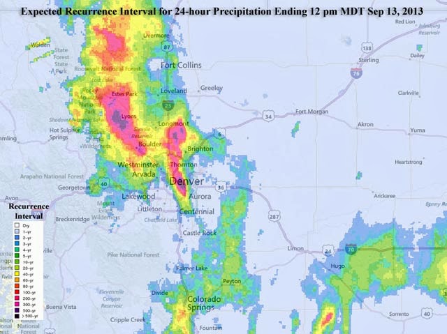
And here is a “recurrence interval.” Have you ever heard the term “100-year-flood”? Well, it looks like this event was closer to the 1-in-1,000 year category in some places, meaning it has a 0.1 % chance of occurring any specific year.
I used Luke Madaus’ Looking Aloft blog, an article written by The Weather Network, and, as mentioned before, Jeff Masters’ Wunderblog as my primary sources of information to write this blog. You should definitely follow Luke’s blog… he’s a UW atmospheric sciences graduate student who was a TA in the 101 class I took with Cliff Mass fall quarter freshman year. He knows his stuff AND is a really good writer. He, along with Scott Sistek and Cliff Mass, are “there” as far as blogging goes. I’m currently “here,” but I’m working on getting over “there.”
We have a wet weekend ahead of us, but I doubt we’ll be seeing any Bible references in NWS forecast discussions. 🙂

Charlie

